A polaron is a quasiparticle composed of a charge and its accompanying polarization field. A slow moving electron in a dielectric crystal, interacting with lattice ions through long-range forces will permanently be surrounded by a region of lattice polarization and deformation caused by the moving electron. Moving through the crystal, the electron carries the lattice distortion with it, thus one speaks of a cloud of phonons accompanying the electron.
The Fröhlich polaron model is one of the simplest examples of a Quantum Field Theoretical problem, as it basically consists of one single fermion interacting with a scalar bosonic field. The polaron model results in a series expansion that can be expressed as a series of diagrams. A 4th order diagram could look like the following:
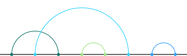
Here we have electron propagators expressed in the bottom dark line (9 electron propagators in total) and phonon propagators with the different colors expressed as arcs (4 phonon propagators). Some of the phonon propagators could be crossing, some could sit under a bigger propagator and some might just be alone and non-crossing.
What I am basically after is the Green's function of the Polaron. A certain diagram represents a term in the (infinite) sum that is the Green's function. Such a term is a product of electron propagators, vertex amplitudes and phonon propagators. After all we have
which is the free electron propagator. For the phonon propagator we have a similar expressions,
where ωp is just a constant as μ before. Finally the vertex amplitude (squared, because we will only have pairs of vertices) looks like
The simulation then basically tries to change the order of the diagram by adding or removing a phonon propagator. We make the restriction that only non-crossing arcs can be removed. Therefore we also just add non-crossing arcs. This gives us a much better performance in our code, since we do not need to compute the full diagram before and afterwards, but just the difference. This difference is computed quite fast.
However, this method requires another action to be implemented: swap. We randomly select two neighboring nodes, which are not connected and connect them. The fourth action is extending / changing the time of the diagram.
Building the code is possible by using the make program. In order to build the application you just have to use the following line in the shell:
make all
If you want to have more output (but this means: A LOT MORE), then you should go for the debug build. This one can be created by using the following command:
make debug
The code comes with a custom random number generator, which is based on the MWC algorithm. The file random.c contains some functions that might help. The functions can generate continuous, discrete, exponential and normal distributed random numbers. The MWC method is known for a very fast generation of sequences of PRN with vast periods, ranging from around 260 to 22000000.
Download polaron.tar.gz (6 kB)
Additionally to the code I've written a little JavaScript to demonstrate that the swap operator is actually able to generate all possible diagrams. A webpage that includes this JavaScript (with an asynchronous webworker) can be found under html5.florian-rappl.de/Polaron/.
This JavaScript visualizes the found diagrams with the help of the HTML5 canvas element. The resulting graphics can be saved on the hard drive.